Archimed 2: ART-LidART

Archimed 2 is an implementation of a raytracing-based simulation program. It consists in tracing the path of light through a scene (e.g. a forest) in order to simulate a satellital lidar waveform, or to compute the radiative balance of a group of plants. In january 2013 these two applications are integrated in simeo: A scene can be built, then exported via the Archimed 2 plugin.

See the ART model development documentation (fr) by R. Cresson
See the Simeo / ART-Archimed2 (jan 2013) tutorial.
See the Simeo / Lidar-Archimed2 (jan 2013) tutorial.

The software can compute the radiative balance of the exported scene. The solar contribution is modelisated with a 46-directions turtle (truncated icosahedron). Light is emitted in each direction with an intensity which is function of the wanted simulated time period. The radiative balance of the vegetation can be performed on the entire scene, or on a used-specified plot.

How to use the Radiative Balance simulation plugin in simeo? The sun parametrization is the same as Archimed-1. But there is some settings specific to the ART raytracing engine:

The threshold coefficient sets the ray intensity level below which its propagation stops. The intensity threshold for one ray is computed from the mean energy of the 46 directions, the total number of rays, and the given threshold coefficient. In fact, the threshold coefficient represents, in proportion of the mean energy of the 46-directions, the value below wich the retrodiffusion is processed.

The maximum ray path length is simply the maximum distance that a ray can travel in the scene.

The space splitting sets the size of the 3D regular grid which is used to partition the scene. This leads to a faster process, but the scene initialization is slow. A little space partition means that computing would be slow by the number of scene objects. A too big space partition could slow the process, allocating too much memory compared to the scene objects number. This parameter depends of your hardware configuration.

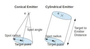
The software can simulate the lidar signal impulse response of the exported scene. The lidar instrument can be modeled as a conical/cylindrical beam: Emitted rays can be parallel (cylindrical emitter) or not (conical emitter) and received light shots are detected when they are is a given field of view (conical). Different parameters of the emitter and the sensor can be set.

How to use the lidar plugin with simeo?

The user must specify the Lidar instrument parameters, via this panel:

The input parameters are:

• The target coordinates (XYZ, in meters)
• The distance between the target and the lidar sensor (in meters)
• The lidar azimuth angle (in degrees)
• The lidar elevation angle (in degrees)
• The type of simulated emitter: Parallel or Conical. When the “parallel” emitter is checked, the incoming rays are parallel. When the “conical” emitter is checked, rays are emitted from a ponctual source so incomming rays are not parallel. When the “parallel” emiter is checked, the user must specify the spot radius (in meters) at the distance of the target. When the “conical” emitter is checked, the user can specify the spot angle (in degrees) or the spot radius (in meters) at the distance of the target.
• The emitter power (in W): it represents the total amount of power for every rays casted from the source.
• The emitter number of different rays (i.e. different orientation and different origin) which are casted from the emitter.
• The sensor gain is the amplification of the received signal by the sensor
• The sensor field of view radius: The sensor can detect only enlighted points which are in a specific range.
• The sensor resolution (is the sensor sampling distance)

The output parameters are:

• Output path: Path for file results export
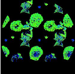
• Emitter image on/off: display the 'emitter image': For each ray (i,j) sent from the emitter, the value of the pixel (i,j) is the total amount of returned intensity to the sensor.
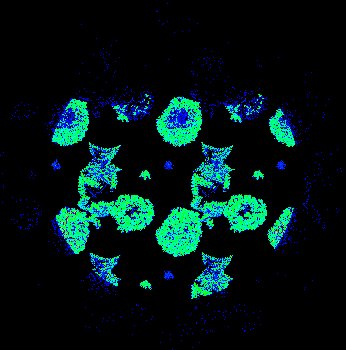
• Sensor image on/off: display the 'sensor image': For each scattering process in the scene (i.e. each ray scattering), the returning intensity to the sensor is computed. The location of each shot is sampled in the sensor's direction (2d, angular) and each returning energy is added in the sampled pixel.
• Smoothing Width: Once the images are obtained, they are filtered with a mean filter of the specified size in order to reduce the noise.

Remark:

• Output images dimensions are linked to the emitter number of rays.

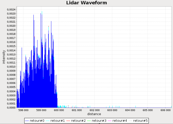
Results of the simulation The lidar impulse response can be viewed as a 2D plot (energy vs distances) and the signal is exported in a .csv file.

The .csv file contains each return, associating an energy value (float) and a distance in meters (float). The user must be attentive to this explaination: With a real lidar instrument, the obtained data is the total amount of energy received during the time (or along the distance). This data is obtained in summing of all simulated intensities at each return order (for line i, sum of columns 1 to N, N being the maximum return order). Indeed, a true lidar instrument does not deliver one intensity for return 0, one other for return 1, one other for return 2, etc. Here, returning intensities are returned for each order because it is an accessible data wich is part of the simulation process.

Two images can also be displayed (optional):

1. The view from the emitter (each emitting cell is filled with the value corresponding to the scattered energy of the rays casted from this cell)
2. The view from the sensor (each sensor cell is filled with the value corresponding to the total scattered energy of the incoming rays on this cell)

See also the animation “lidar.gif” in screenshots